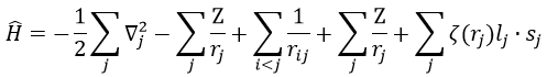
The presence of a second electron induces a term of repulsion between electrons.

This term is positive so it increases the energy of the orbitals. The rest of the equation is similar to the Hamiltonian of the hydrogen. We can compare the energy of the orbitals with those two models.

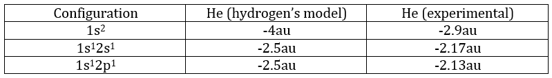
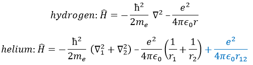
The repulsion is large in the 1s orbital wherein the electrons are close to each other (the radius being small). For instance, the energy of the orbital 1s² of the Helium is at -2.9au (atomic units). If we calculate the energy without the repulsion term, i.e. as a monoelectronic atom (Ĥ= Ĥ₁ + Ĥ₂), we find -4au (E₁=E₂=-Z²/2n²=2au). Another consequence is that the orbitals s and p don’t have the same energy anymore. The configurations 1s¹2s¹ has an energy of -2.17au and the configuration 1s¹2p¹ an energy of -2.13au.

We can separate the Hamiltonian into one monoelectronic Hamiltonian term and the term of repulsion between the electrons.

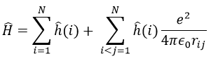
ĥ(i) is the monoelectronic Hamiltonian of one electron.  We sum up the terms for all the electrons to obtain the Hamiltonian. To resume, the repulsion spreads the degenerated orbitals from the monoatomic model.

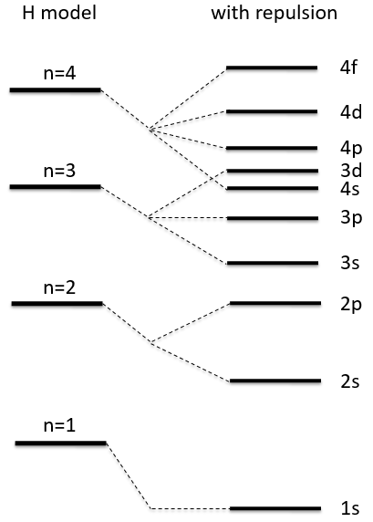
The repulsion can be large enough to have an orbital of level n+1 of lower energy than an orbital of n. It is the case for orbitals d and f and it is why we use the following technique to fill the orbitals with electrons:

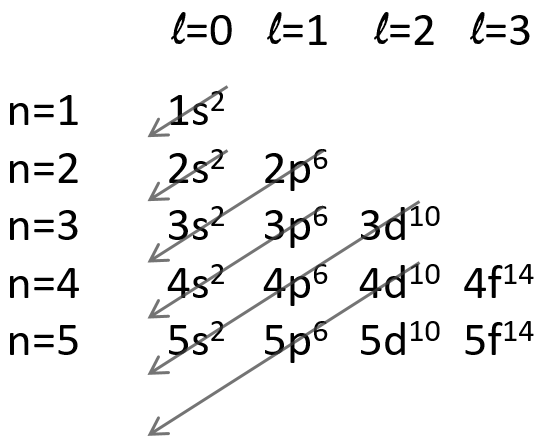
The 4s orbital is thus filled before the 3d orbital.

The operators that commute are simply the sum of the operators applied to the electrons independently (but perturbed by the repulsions). We write these operators with a lower case to denote them from the global operators (Ĥ→ĥ, Ŝ→ŝ, …).

The electrons are indistinguishable. It means that if we exchange an electron of an atom with another electron of the atom on the same orbital or on a different orbital, the atom remains unchanged. We can thus introduce a permutation operator P_ij that commutes with the Hamiltonian Ĥ and the proper value of which is ±1. This last affirmation is true because we get back to the initial conditions if we apply the permutation operator P_ij twice. The identity operator Ê is the operator with which nothing changes: ÊΨ=Ψ.

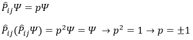
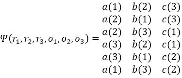
The value of p is imposed by the type of particle. Bosons have a integer spin and p_boson=1. Fermions have half-integer spins and p_fermion=-1. Electrons are thus fermions. Some nuclei are bosons and some are fermions. In an atom with N electrons, N! permutations of electrons are possible. For instance, the lithium has 3 electrons with spherical coordinates (r₁, σ ₁), (r₂, σ₂) and (r₃, σ ₃) (considering the orbitals 1s and 2s) that can be permuted between 3 spots a, b and c. There are 6 possible permutations 6=3! = 3x2x1): P₁₂, P₁₃, P₂₃, (P₁₃,P₁₂), (P₁₃,P₂₃) and Ê.

We don’t know which electron is in which spot (a, b or c). The wave function Ψ is one of the functions

To write the wave function we use the determinant of Slater which is a combination of the possible states.

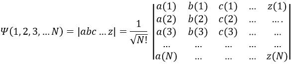
with a, b, c, …, z are the spin orbitals.

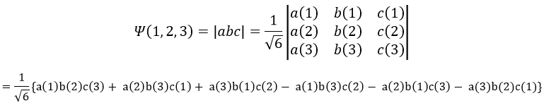
In mathematics, a determinant is read in diagonal. The elements of the diagonals (from top left to bottom right) are multiplied and the diagonals are summed up. Then we deduce the diagonals in the other way (from top right to bottom left). In the case of the lithium we have

The determinant of Slater has a few properties:

• if we exchange two lines or two columns, the sign of the determinant changes.
• if two columns are identical, the determinant equals 0.

It can be translated by the law of Fermi: 2 electrons must differ by at least one quantic number.

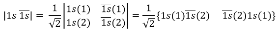
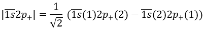
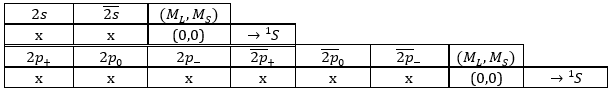
Let’s apply this to the helium and a few of its excited states. He has 2 electrons that are distributed on the 1s orbital in its ground state. There can be two electrons on this orbitals if they have different spins (1/2 and -1/2). In the notation of Slater, the spin is indicated by the presence of a line above the orbital if the spin=-1/2.

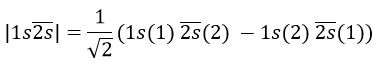
For the excited state wherein one electrons jumped to the orbital 2s, there are 4 possible states depending on the spin of the electrons:

For instance,

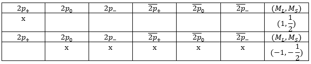
If instead the electron jumped to the 2p orbital, there are 12 possible states:

For instance,

Coupling of Russel-Saunders

This coupling is also called the L-S coupling. We consider it for multi-electron atoms with weak spin-orbit couplings. In this case, the orbital angular moments of the individual electrons add to form a resultant orbital angular momentum L and the same is true for the spin moments to form a spin angular moment S. L and S combine to form the total angular moment J.

J=L+S

The resultant of two vectors is their sum. If we consider two operators Ĵ₁ and Ĵ₂ (which can be L and S), their resultant Ĵ = Ĵ₁+ Ĵ₂.

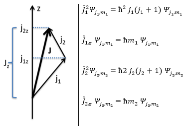
Ĵ_z is simply equal to the sum of Ĵ_1z and Ĵ_2z and Ĵ² is the development of the square of the sum

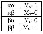
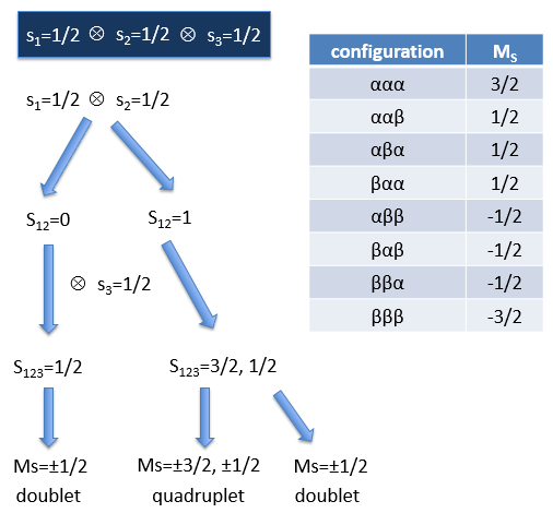
We can look at the coupling between the electrons in He. The electrons have a spin s=1/2 and m_s=±1/2. Let’s say that m_s=1/2 is the state α and that m_s=-1/2 is the state β. The coupling can be αα, αβ, βα or ββ coupling. The coupled M_s=m_s1+m_s2 can thus be equal to 1, 0, 0 or -1. We write these values in a table. I insist on the fact that M_s=0 is degenerated.

To know the resulting states of the coupling between the electrons, we take the largest S=s₁+s₂ and look for its M_s in the results of the coupling. It is S_max=1 with M_s=-1, 0 and 1. We discard these values of M_s from the 4 couplings that we obtained earlier. If there are one or more remaining M_s in the table, we do the same for S=S_max-1, etc. Here, there is one last M_s=0 that comes from S=0. The 4 couplings correspond thus to a singlet state (S=0 and M_s=0) and 1 triplet state (S=1 and M_s=1, 0 or -1). S goes from ∣s₁+s₂∣ to ∣s₁-s₂∣ by step of 1. The multiplicity is equal to 2S+1. The difference between the states is always by step of ΔS=1 and ΔM_s=1. The states can be represented this way:

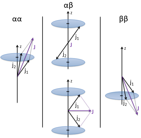
Note that the vectors for M_s=1 or M_s=-1 are not two times the length of the vectors for ms1 and ms2. The vertical component is. Note too that the resulting vector for M_s=0 may have a nonzero length (S=1).

If 3 electrons are coupled, we proceed step by step. First we do the coupling between two electrons. As previously we obtain two different states, S₁₂=0 (singlet) and S₁₂=1 (triplet). There is no need yet to determine Ms. The last electron is coupled next to the two possible states S₁₂. The coupling with the singlet S₁₂=0⊗s₃=1/2 gives S₁₂₃=1/2. It is a doublet (M_s=1/2 or M_s=-1/2, remember that ΔM_s=1 between ∣S₁₂+s₃∣ to ∣S₁₂-s₃∣). The coupling S₁₂=1⊗s₃=1/2 gives a total of S₁₂₃=3/2 (1+1/2), leading to two states S₁₂₃=3/2 and S₁₂₃=1/2 (ΔS=1). It means that there is a quadruplet (2(3/2)+1=2) and a doublet (2(1/2)+1=4). In total, there are 2ⁿ=8 possible states, n being the number of electrons.

In the case of degenerated orbitals as the orbitals p or d, the amount of configurations is larger (see the part about the determinant of Slater) but the method is identical and is also applied to the quantic number l. Let’s take a few examples: the electronic configurations (1s)¹(2s)¹, (1s)¹(2p)¹ and (2p)¹(3p)¹.

Configuration (1s)¹(2s)¹

The degeneration is 4: the two electron can have a positive or a negative spin (α or β). We have thus 2×2=4 degenerated configurations:

There is only one value for the orbital number L=0: l_1s=0⊗l_2s=0. As a result, M_L=0. As we have seen above, the coupling between two electrons s_1S=1/2⊗s_2s=1/2→S=1, 0 gives one singlet (S=0, degeneration =1) and one triplet (S=1, deg=3).

We write the electronic term depending on L and S. L gives a capital letter S, P, D, F the same way n gives s, p, d, f. The electronic degeneration is written as an exponent before the orbital letter. The electronic terms for the configuration (1s)¹(2s)¹ are thus ¹S, ³S. The degeneration of the terms is the multiplication of the degeneration of L and S and we sum up the degeneration of the electronic terms: 1.1 (for ¹S) +1.3 (for ³S) = 4. We have thus a concordance between the degeneration of the terms and the degeneration of configuration.

Configuration (1s)¹(2p)¹

The degeneration is 12 in this case: both electrons can have a positive or negative spin (α or β) but the 2p electron can be on 3 different orbitals (2p_–, 2p₀ or 2p₊). We have thus (1.2).(3.2)=12 degenerated configurations (written earlier in the chapter).

The coupling l_1s=0⊗l_2p=1 gives L=1 (M_L=-1, 0, 1). There is no L=0 here: if we look at the details of the coupling.

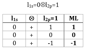
We find the M_L’s of L=1 but once they are discarded, there is no other M_L. There is thus no L=0. An easier way to know it is that L goes from ∣l₁=l₂∣ (=1) to ∣l₁-l₂∣ (=1-0=1).

As L=1, the electronic terms will be ^xP with x=1 and 3 from the spin. As always, the coupling between two electrons gives a triplet and a singlet. The electronic terms are thus ¹P, ³P with a degeneration (3.1)+(3.3)=12.

Configuration (2p)¹(3p)¹

The degeneration is 36 ((3.2).(3.2)): 3 orbitals with 2 possible spins for each electron. The coupling l_2p=1⊗l_3p=1 gives L=2 (M_L=-2, -1, 0, 1, 2), L=1 (M_L=-1, 0, 1) and L=0 (M_L=0). The coupling of spins gives one singlet and one triplet as usual. We have thus the electronic terms

¹S, ¹P, ¹D, ³S, ³P, ³D that can also be written as ¹(S, P, D), ³(S, P, D) or even ^1,3(S, P, D)

The degeneration are respectively (1.1), (3.1), (5.1), (1.3), (3.3) and (5.3) for a total of 36.

If we want to couple a third electron, we obtain the electronic terms by coupling separately the electronic terms if the electrons are not equivalent. For instance, if we add a 3d electron (²D) to the 2p3p electrons, we proceed this way:

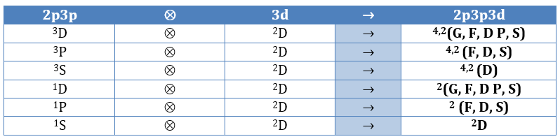
One can see that some electronic terms are obtained several times (²F for instance). Those terms are not identical and have not the same energy because they come from different couplings.

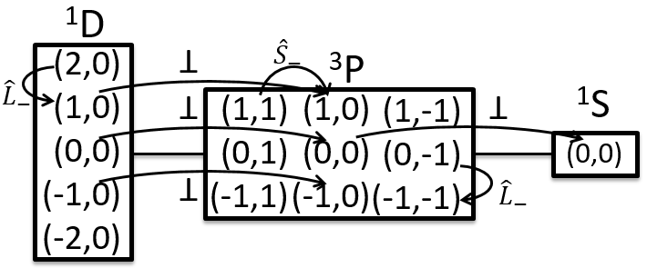
In the case of equivalent electrons, the amount of states is more limited. For instance we had 36 possibilities for the 2p3p configuration. This amount drops to 15 for the 2p² configuration. This amount is equal to X!/(X-N)!N! where X is the degeneration of the state and N the number of electrons. In our case, 2p², N=2 and X=6 for the orbital 2p: there are 3 orbitals (2p₊, 2p₀ and 2p_–) and 2 spins. There are thus 6.5/2=15 possibilities. To determine the electronic terms of this coupling, we will make a list of the 15 possibilities and identify each one by the couple (M_L,M_S). To do so we draw a table with a column for each one of the 6 states and we put pairs of electrons together. In a seventh column, we write down the (M_L, M_S) of the couple of electrons.

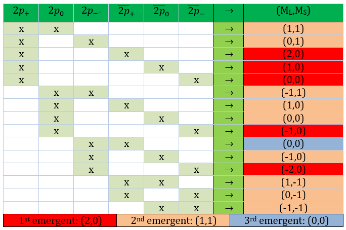
Once it is done, we seek for the emergents. An emergent is one couple of projections that is unique. We take the one with the largest values, i.e. (2,0) in this case and we determine the electronic term from which the pair comes. M_L=2 means that L=2 and M_S=0 means that S=0. The corresponding electronic term is ¹D that has a degeneration of 5. As a consequence we will find 5 pairs of projections in the table that come from the electronic term ¹D.

We can remove them from the list and look for another emergent: (1,1). The corresponding electronic term is ³P with a degeneration of 9. From the 15 possibilities, 14 correspond to 2 electronic terms (³P and ¹D). The last emergent is (0,0), what corresponds to the electronic term ¹S. The electronic terms of the configuration 2p² are thus ¹D ³P ¹S. In comparison with inequivalent electrons (2p3p), the ³D, ¹P and ³S terms disappeared. Also note that several pairs were several times in the list and we randomly selected which one corresponds to which electronic term. For instance, we don’t know which (1,0) comes from ¹D or from ³P.

In terms of energy, the rules of Hund tell us that the term with the highest M_S is the most stable. If there are identical M_S projections, then the highest M_L is the most stable. For instance, the ³P coupling of 2p² has a lower energy than ¹D itself lower than ¹S.

Here come two properties of the L-S coupling:

• Complete orbitals are all ¹S:

As a result, they do not modify the other orbitals. Note that even if they do not perturb the other orbitals, they do contribute to the energy of the electronic states.

• A “hole” (the absence of electron) in one orbital gives the opposite signs of M_L and M_S than the presence of this electron. For instance

But the sign doesn’t change the state. As a result, the carbon (2p²) and the oxygen (2p⁴) have the same state ²P.

Spin-orbit coupling

The magnetic moment induced by the spin of the electron interacts with the magnetic field induced by the electric current resulting from its orbital movement. This relativist effect induces a further separation of the states and an additional term in the Hamiltonian.

The coupling introduces a new observable J=L+S

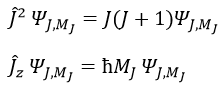
J goes from L+S to ∣L-S∣ by step of 1. Considering this, [Ĥ,L²] and [Ĥ,Ŝ²]≠0 but [Ĥ,Ĵ²]=0.

The relativist effects grow with the atomic number of the atom: the larger the atomic number, the heavier the nucleus. Its charge increases as well meaning that the electrons have to revolve faster to compensate.

Energy of the states

The energy of the states can be found from the equation of Schrödinger

From that, we can write

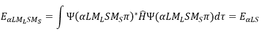
The energy is thus the average value of Ĥ. To determine it, we start from a linear combination of determinants of Slater (M_L,M_S). An emergent determinant of Slater always gives a proper function. From this point, we can apply operators L₊, L_–, Ŝ₊ or Ŝ_– to increase/decrease the value of M_L or M_S and find their energy.

We do it for each state that has at least an emergent. If there is no emergent, we can apply the rules of orthogonality: 2 wave functions that differ by at least one proper value of operators that commute together are orthogonal. Eventually, the proper functions are normalised.

With this method, the energies of the states can be found. One simple example says more than a thousand words. The coupling of two electrons gives a singlet (S=0, MS=0) and a triplet (S=1, M_S=1, 0, -1). We will place the values of M_S in boxes for S=1 and S=0, as shown below.

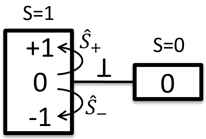
An emergent is found for M_S=1 (S=1) so we can find the wave function Ψ_S=1,Ms=1 (the state αα). We also have the wave function of Ψ_1,-1 (the state ββ) because it is an emergent too.

To obtain the wave function of the state M_S=0, we apply the operator of descent Ŝ_– on Ψ_1,1 (we could have applied Ŝ₊ on Ψ_1,-1 instead).

One electron in the α state is thus now in the β state. We need to norm the function. To do so, we must have the norm N equal to

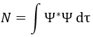
Applied here, we have

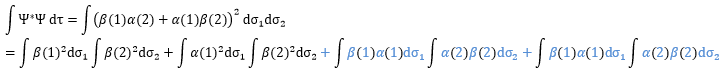
The orbitals are orthonormal, meaning that the integrals equal 1 if the two terms of the integrant are identical and zero if they are different: ∫αα=1, ∫ββ=1, ∫αβ=0, ∫βα=0. The cross terms of the square (in blue) are thus equal to zero and the others equal 1.

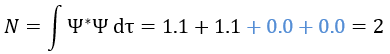
As a result,

To obtain the wave function of the singlet, we can use the property of orthogonality between Ψ_1,0 and Ψ_0,0. Posing β(1)α(2)=x and α(1)β(2)=y,

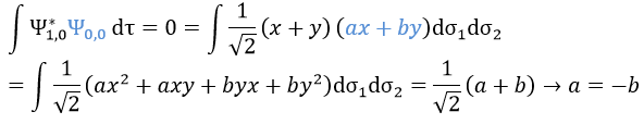
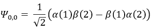
Meaning that, once normed,

The same method can be applied on more complex cases. For instance with two 2p electrons: