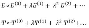
We have seen quite a lot of new stuff up to now. We described monoelectronic and polyelectronic atoms and developed the description to molecules through the approximation of Born-Oppenheimer, the theory of groups and the CSOC. All of this teaches us how orbitals are and how they change during a reaction. Yet, we did not find the energies of the orbitals and can’t say which one is more stable than the others. The general equation is, as seen at the beginning of the course,
![]()
From the wave function we want to determine the energy of the orbitals but we can’t solve the equation exactly except for systems with one electron. For other species, we can only find an approached solution. To obtain it, we use the theory of perturbations or the method of variations.
Theory of perturbations
We can apply this theory to states that are independent of the time, i.e. stationary states. We can approximate the Hamiltonian and the energy of one state if this state is the result of a small perturbation λ of a state the solutions of which are known (Ĥ(0), E0).
![]()
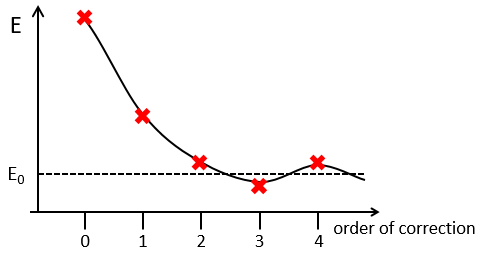
The solutions are then expressed as a series of correction to the model at order zero.
The corrections are calculated from the solutions at the order 0. For instance, the correction of order 1 are
![]()
The corrections usually decrease in intensity with their order but they will always approach the approximation from the exact solution. Note that we can go beneath the exact solution.
Method of variations
To find the exact energy, we use a trial wavefunction. This function has a known form but will probably not give the exact energy but will give us a superior born for the exact energy. Next, we modify the parameters of the trial wavefunction to obtain a better approximation of the energy. Unlike the method of perturbation, we can’t go beneath the exact energy with the method of variations. Each time we modify the parameters, we obtain a solution of lower energy and we approach the exact value of the energy. For instance if we chose a wavefunction with two parameters α and β. We can try to improve the values of the parameters to obtain the best possible approximation.
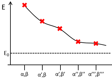
We reach an optimal estimation when the energy does not vary anymore when we change the parameters, i.e. when dE/dparameters=0.
Application to the helium
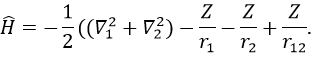
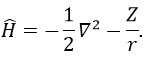
We will apply those two methods to estimate the energy of the helium. The exact solution is E=-2.903u.a. and the complete Hamiltonian is
One model the solution of which is known is the hydrogenous model:
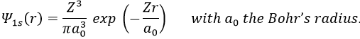
The solution of this model for 1 electron is
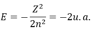
with Z the atomic mass and the quantic number n. As there are two electrons in the helium, we simply multiply the energy by 2 to obtain a first approximation from the hydrogenous model:
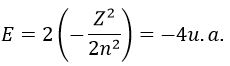
This approximation is far from the exact solution and overestimates the stability of the atom because we did not take the repulsion between electrons into account (the +1/r12 term).
The theory of the perturbation will start from this model and introduce the repulsion term as a pertubation of the model:
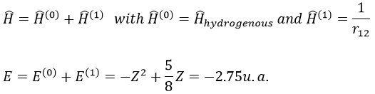
This estimation is way better than the hydrogenous model alone.
The method of variations is slightly different as we choose a wave function Ψ that depends on a few parameters that we may vary. As for the theory of perturbations, we select the hydrogenous wave function
As there are two electrons in the helium, we use a combination of two wave functions:
![]()
The parameter that we will vary is the effective charge Z=Zeff. One part of the charge of the nucleus is indeed hidden to one electron by the second electron.
From the chosen wave function, we find an equation for the energy that depends on Z
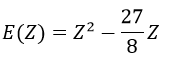
We optimise the parameter to obtain the best approximation that we can, such as dE/dZ=0. Solving this, we find
![]()
We apply this particular value of Z to the equation for the energy to find
![]()
This result is close to the exact solution.
Principle of linear variation: linear combination of atomic orbitals (LCAO)
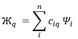
In this method, we assume that Ж can be expressed as a linear combination of a base of functions {Ψ1, Ψ2, …}
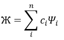
where ci is the variational parameter associated to the wave function Ψi. These coefficients are adjusted to approximate the exact energy. For more simplicity, let’s take an example in which Ж is a linear combination of two wave functions Ψ1 and Ψ2.
![]()
It is corresponding to the case of H2:
![]()
The Hamiltonian is
![]()
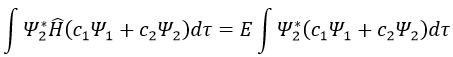
Next we multiply this equation by Ψ1* and integer it over tau:
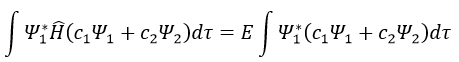
We can do the same with Ψ2*:
Now, we introduce Hij and Sij such as
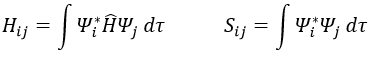
The previous integrals can be written
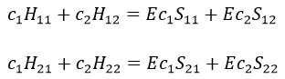
or
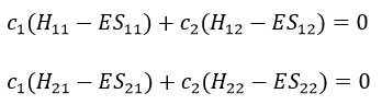
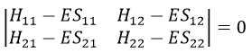
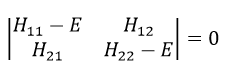
This system of two equations can be written as a 2×2 secular determinant
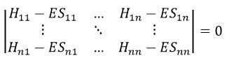
In a general way, it forms a n by n secular determinant if there are n wave functions (or particles)
The n solutions of the secular determinant give the n most stable states of energy of the system. If we inject one of the energies E=Eq in the system, we obtain the optimised coefficients {ciq} related to the state q.
If the base is orthonormal, then
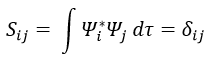
And then
If the base is complete, the linear combination corresponds to the exact solution due to the theorem of superposition (Quantum superposition is a fundamental principle of quantum mechanics. It states that, much like waves in classical physics, any two (or more) quantum states can be added together (“superposed”) and the result will be another valid quantum state; and conversely, that every quantum state can be represented as a sum of two or more other distinct states). The more the base is complete, the more one tends to the exact solution.
Method of Hartee-Fock
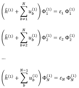
This method is an application of the variational method in which the trial wave function is a normalised determinant of Slater Ж = ∣ Φ 1 Φ 2 Φ 3… Φ N ∣. We try to minimise the energy of the orbitals (∂E/∂Φi=0) and to keep them orthonormal. We obtain a system of N coupled equations of Hartree-Fock that describe the movement of one electron in the averaged field ub created by the other electrons, such as
where εa is the HF energy of the molecular orbital Ψa. If we introduce the operator of Fock
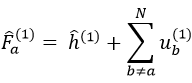
we can rewrite the system of N equations as
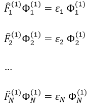
or on one line:
![]()
This equation only depends on the position and the movement of one electron, the effect of the other electrons being averaged. As the averaged field is determined by the orbitals that we are looking for, we have to solve the system of equations by iterations, starting from a set of orbitals of trial.
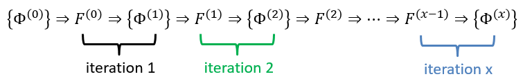
The convergence is guaranteed by the variational principle. In practice, we develop each orbital as a linear combination of Gaussian atomic orbitals centred on the nuclei. Then we iterate.